NLP Methods

import pandas as pd
import plotly.express as px
import plotly.io as pio
pio.renderers.default = "vscode"
from pyspark.sql import SparkSession
from pyspark.sql.functions import split, explode, col, regexp_replace, transform, isnan

spark = SparkSession.builder.appName("LightcastCleanedData").getOrCreate()

# Reload processed data
df_cleaned = spark.read.option("header", "true").option("inferSchema", "true").option("multiLine","true").csv("data/lightcast_cleaned.csv")

# View data structures and samples
df_cleaned.show(5)

Extracting Key Terms from Job Descriptions Using TF-IDF

We start by extracting the job description text from the “BODY” column and convert it into a Pandas DataFrame for easier text processing. To clean it up a bit, we remove line breaks so that the text becomes more uniform and easier to analyze. Then, we apply TF-IDF (Term Frequency-Inverse Document Frequency), which helps us identify and quantify the most important words across all descriptions, ignoring common English stop words. This transformation converts the text into a numerical format, capturing how relevant each word is in a particular document compared to the whole collection.

from sklearn.feature_extraction.text import TfidfVectorizer

# Convert to Pandas DataFrame, taking only BODY columns
body_df = df_cleaned.select("BODY").dropna().toPandas()

# Clear text
body_df["BODY"] = body_df["BODY"].str.replace(r'\n|\r', ' ', regex=True)

# TF-IDF extract

tfidf_vectorizer = TfidfVectorizer(max_features=1000, stop_words='english')
X_tfidf = tfidf_vectorizer.fit_transform(body_df["BODY"])

Visualizing Job Clusters with Word Clouds

We applied KMeans clustering to the TF-IDF features of job descriptions to group similar postings into four distinct clusters. Each job was assigned a cluster label, which we then used to explore the top terms that defined each group. By extracting the most influential keywords from each cluster’s TF-IDF centroid, we generated word clouds to visualize the dominant language and themes within each cluster. These word clouds help us quickly grasp the unique focus of different groups, whether it’s technical, managerial, or creative roles, based on the language used in job descriptions.

Clustering TF-IDF features with K-Means

from sklearn.cluster import KMeans

k = 4
kmeans = KMeans(n_clusters=k, random_state=42)
clusters = kmeans.fit_predict(X_tfidf)

# Add the clustering results to the original DataFrame
body_df["cluster"] = clusters

Generate word clouds for each cluster

from wordcloud import WordCloud
import matplotlib.pyplot as plt
import numpy as np
import os

# Get a glossary
terms = tfidf_vectorizer.get_feature_names_out()

# Get the top keywords for each clustering center
order_centroids = kmeans.cluster_centers_.argsort()[:, ::-1]

# Create directory
output_dir = "images/wordcloud"
os.makedirs(output_dir, exist_ok=True)

for i in range(k):
    print(f"Generate a word cloud of class {i}...")

    top_terms = [terms[ind] for ind in order_centroids[i, :40]]
    weights = {term: kmeans.cluster_centers_[i][terms.tolist().index(term)] for term in top_terms}

    wordcloud = WordCloud(
        background_color='white',
        width=1600,
        height=800,
        max_font_size=300,
        prefer_horizontal=0.9
    ).generate_from_frequencies(weights)

    plt.figure(figsize=(16, 8))
    plt.imshow(wordcloud, interpolation='bilinear')
    plt.axis("off")
    plt.title(f"Cluster {i} Top Terms", fontsize=20)

    # Save the image to the specified directory
    output_path = os.path.join(output_dir, f"cluster_{i}_wordcloud.png")
    plt.savefig(output_path, dpi=300, bbox_inches='tight')
    plt.show()

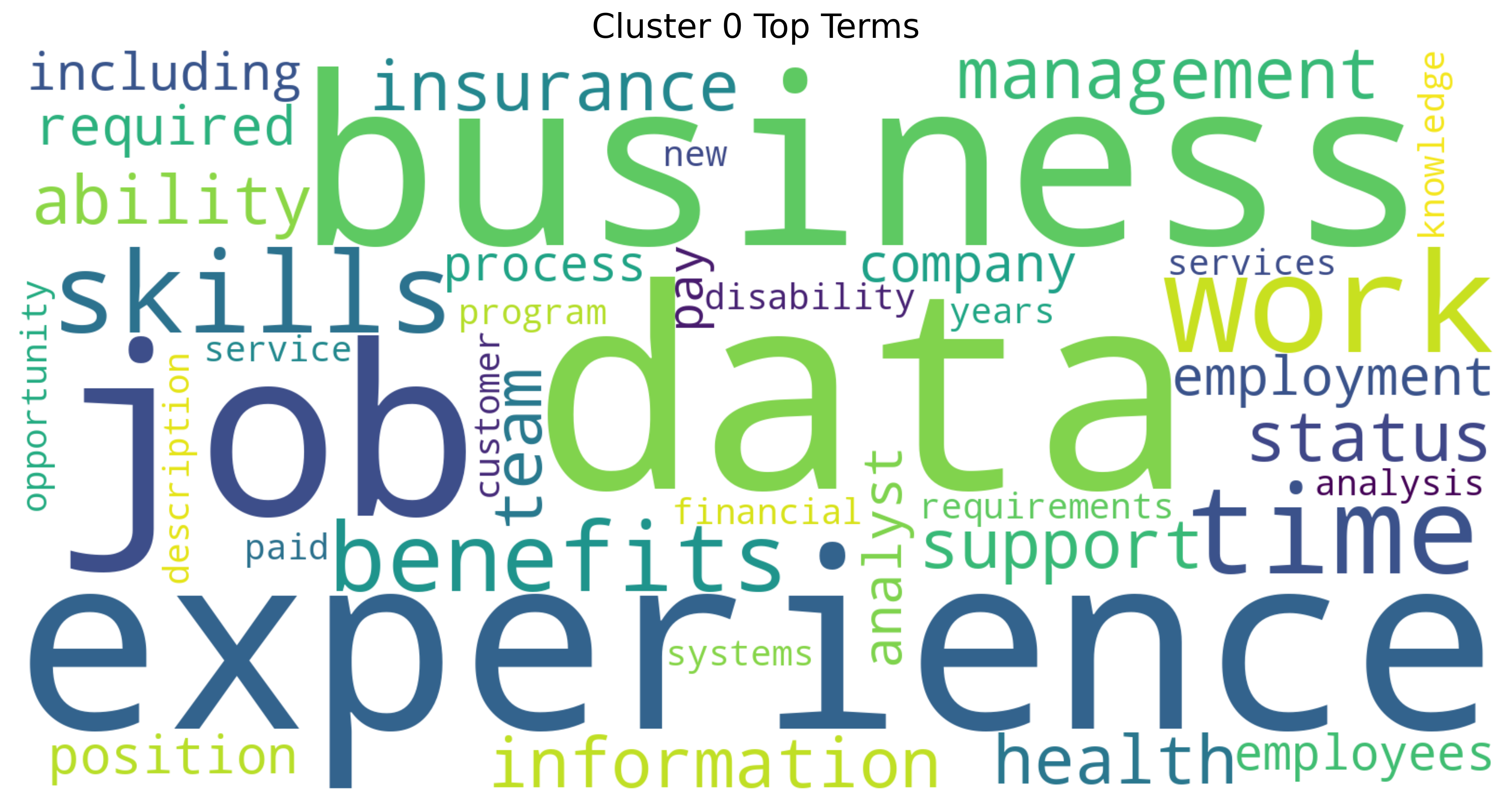
Cluster 0 Word Cloud

Cluster 0 Wordcloud

This word cloud for Cluster 0 highlights a strong focus on job-related themes, with “experience”, “data”, “business”, and “job” standing out the most. It suggests that this cluster centers on professional qualifications, workplace expectations, and the value of skills in data and business environments. Terms related to benefits, insurance, and work-life aspects like “time” and “support” also appear prominently, pointing to both the practical and strategic dimensions of employment (Quan and Raheem (2023)).

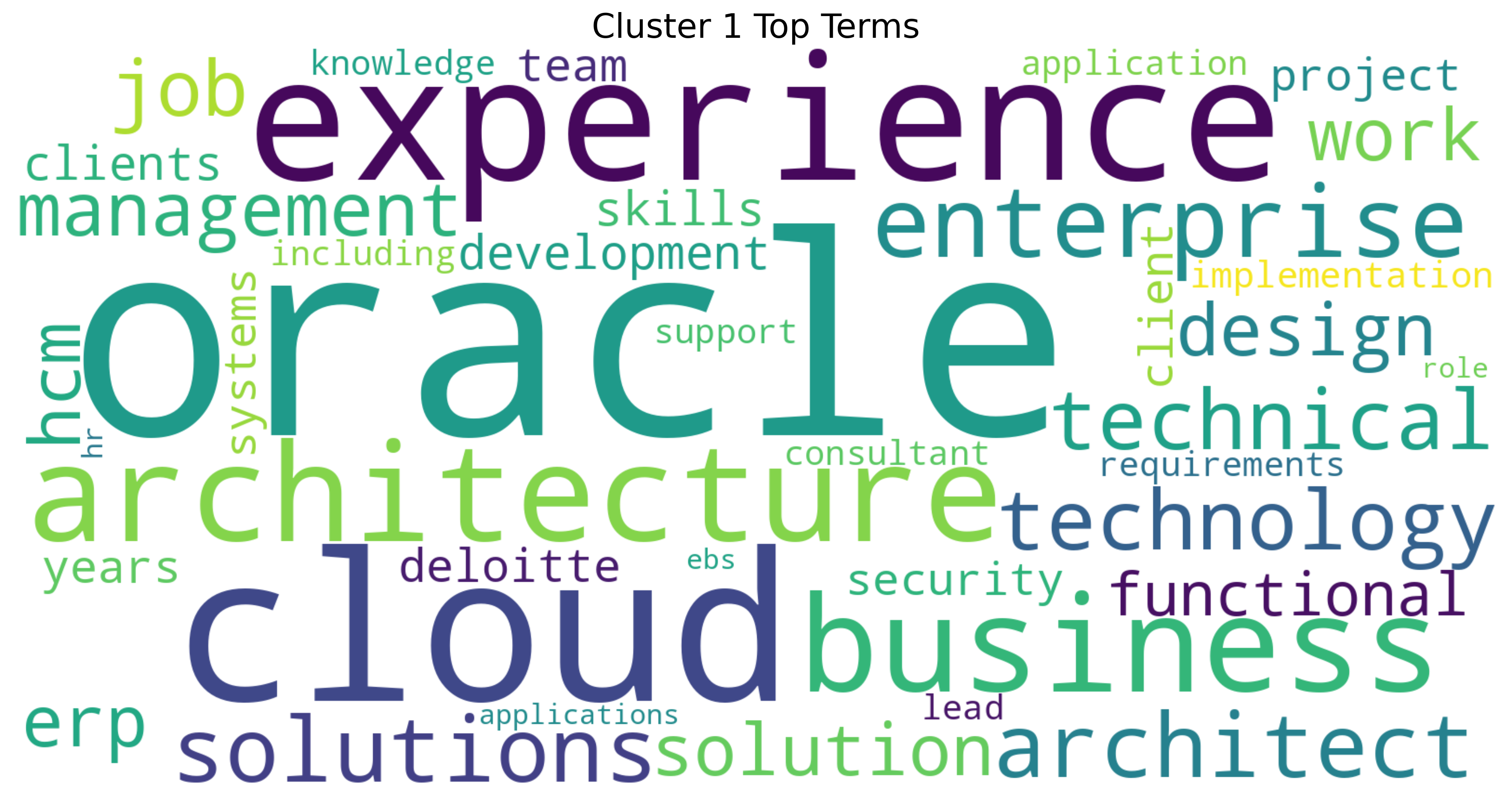
Cluster 1 Word Cloud

Cluster 1 Wordcloud

This word cloud for Cluster 1 revolves around enterprise technology and cloud-based solutions, with strong emphasis on “experience”, “oracle”, “cloud”, and “architecture”. It reflects a technical and strategic domain where roles focus on designing and implementing enterprise systems (Khan et al. (2024)). Terms like “solutions”, “technology”, and “business” suggest a blend of IT expertise and business alignment, especially in environments involving enterprise resource planning (ERP) and cloud infrastructure. The presence of “architect”, “technical”, and “functional”, points to both high-level system design and hands-on implementation know-how.

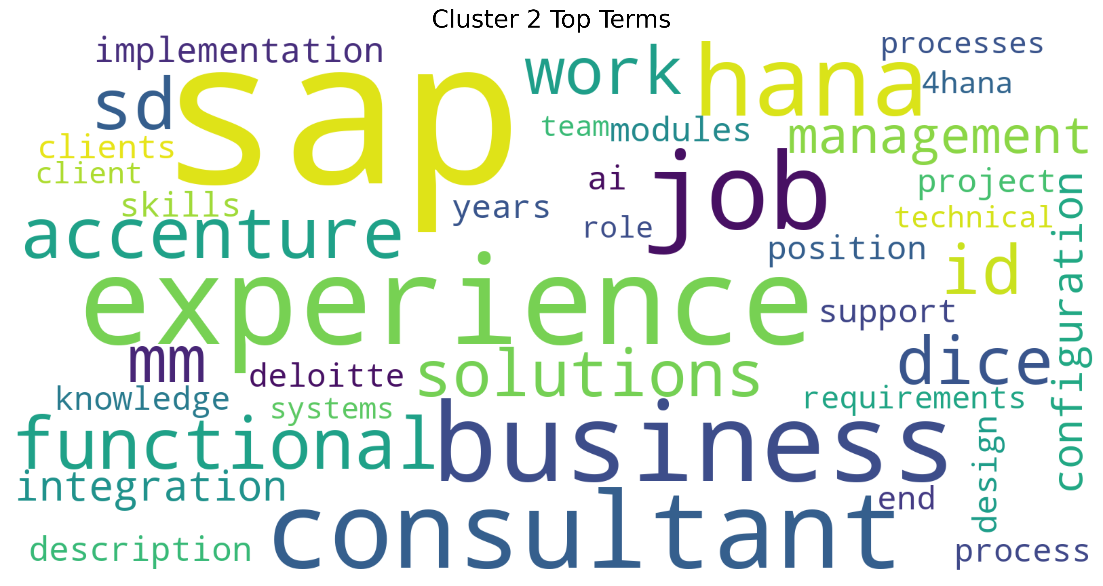
Cluster 2 Word Cloud

Cluster 2 Wordcloud

This word cloud for Cluster 2 reveals a strong focus on IT consulting and enterprise systems, with “SAP”, “experience”, “business”, and “consultant” as dominant terms. It clearly centers on the technical implementation and configuration of SAP solutions (Khan et al. (2024)), with consulting firms like Accenture and Deloitte featured prominently. The presence of terms like “HANA”, “integration”, “functional”, and “implementation” points to specialized SAP modules and project work. This cluster represents the professional ecosystem of SAP consultants who bridge technical expertise with business process knowledge.

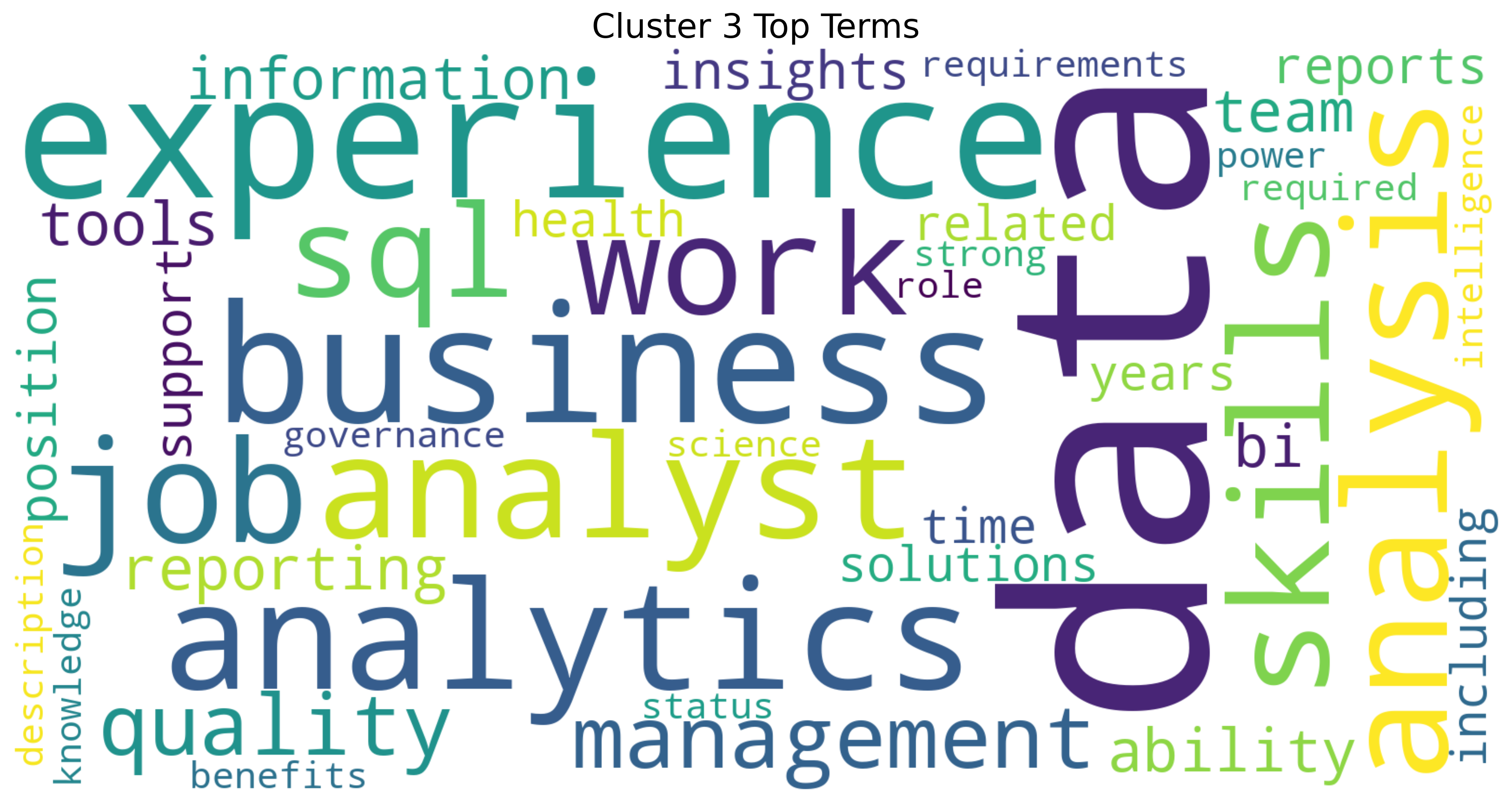
Cluster 3 Word Cloud

Cluster 3 Wordcloud

This word cloud for Cluster 3 showcases the data analytics profession, with “data”, “experience”, “analytics”, and “analysis” dominating the visual. It highlights the business intelligence landscape where SQL skills meet management responsibilities (Quan and Raheem (2023)). Terms like “quality”, “reporting”, and “tools” point to the practical implementation side, while “business” suggests the crucial connection between technical analysis and organizational value. This cluster represents the growing field of data-driven decision making.

Distribution of the number of jobs in each category

import plotly.express as px

fig = px.histogram(body_df, x="cluster", nbins=k, title="Distribution of jobs by theme (cluster)")
fig.write_html("./images/jobs_by_theme.html")
fig.show()

The plot visualizes the distribution of jobs across different clusters. The x-axis shows the cluster categories, while the y-axis displays the count or number of jobs within each cluster. From the plot, we can observe that cluster 0 has the highest number of jobs, indicating that this group is the most prevalent, and also followed by cluster 3. Clusters 1 and 2 have lower counts compared to the other two, suggesting these groups are less represented in the dataset.

Training a SVM & Naive Bayes models using TF-IDF features

We trained two different classifiers, Naive Bayes and Support Vector Machine(SVM), to predict job clusters based on TF-IDF features extracted from job descriptions. By splitting the data into training and testing sets, we evaluated the models’ accuracy in classifying unseen samples. The classification reports provided detailed performance metrics, while a confusion matrix visualized how well the SVM model distinguished between the four clusters. This approach helps us assess the feasibility of using machine learning to automatically categorize job posts based on their content.

Training two classifiers

from sklearn.model_selection import train_test_split
from sklearn.naive_bayes import MultinomialNB
from sklearn.svm import LinearSVC
from sklearn.metrics import classification_report, confusion_matrix
import seaborn as sns

# Using clusters as classification targets
y = body_df["cluster"]

# Splitting the training and test sets
X_train, X_test, y_train, y_test = train_test_split(X_tfidf, y, test_size=0.2, random_state=42)

# Training the Naive Bayes Classifier
nb_model = MultinomialNB()
nb_model.fit(X_train, y_train)
y_pred_nb = nb_model.predict(X_test)

# Training SVM Classifiers
svm_model = LinearSVC()
svm_model.fit(X_train, y_train)
y_pred_svm = svm_model.predict(X_test)

# Evaluate Naive Bayes
print("\n Naive Bayes :")
print(classification_report(y_test, y_pred_nb))

# Evaluate SVM
print("\n SVM :")
print(classification_report(y_test, y_pred_svm))

# Confusion Matrix of SVM
cm = confusion_matrix(y_test, y_pred_svm)
plt.figure(figsize=(6, 5))
sns.heatmap(cm, annot=True, fmt='d', cmap='Blues', xticklabels=range(k), yticklabels=range(k))
plt.xlabel("Predicted")
plt.ylabel("True")
plt.title("SVM confusion matrix")
plt.savefig("images/SVM_confusion_matrix.png", dpi=300, bbox_inches='tight')  
plt.show()

Naive Bayes Result

Naive Bayes

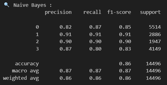
The Naive Bayes classification model shows strong performance across all four job clusters. The model achieves an overall accuracy of 86% across 14,496 samples. Looking at individual clusters, cluster 1 demonstrates the best performance with precision and recall both at 91%, resulting in an F1-score of 0.91 across 2,886 samples. Cluster 2 follows closely with balanced precision and recall at 90% (F1-score of 0.90), though it has the smallest support with only 1,947 samples. Cluster 0, which contains the largest number of samples (5,514), shows good performance with 82% precision and 87% recall. Cluster 3 has slightly lower metrics with 87% precision and 80% recall. The macro average scores of 0.87 across all metrics indicate consistent performance across the different clusters, suggesting the Naive Bayes model effectively captures the distinctive language patterns in each job cluster identified through the previous TF-IDF analysis and K-means clustering.

SVM Result

SVM

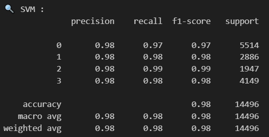
The Support Vector Machine (SVM) model also demonstrates exceptional performance in classifying job postings across all four clusters. With an overall accuracy of 98% on the 14,496 samples, the SVM significantly outperforms the Naive Bayes model. All four clusters show remarkably consistent and high precision scores of 0.98. Cluster 2, despite having the smallest sample size (1,947), achieves the highest performance with 0.99 for both recall and F1-score. Clusters 1 and 3 both maintain excellent 0.98 scores across precision, recall, and F1-score, while Cluster 0 (the largest cluster with 5,514 samples) shows slightly lower but still impressive recall at 0.97. The uniformly high macro and weighted averages (0.98) across all metrics indicate that the SVM model excels at distinguishing between the different job clusters based on their TF-IDF features, making it particularly well-suited for this classification task.

SVM Confusion Matrix

SVM confusion matrix

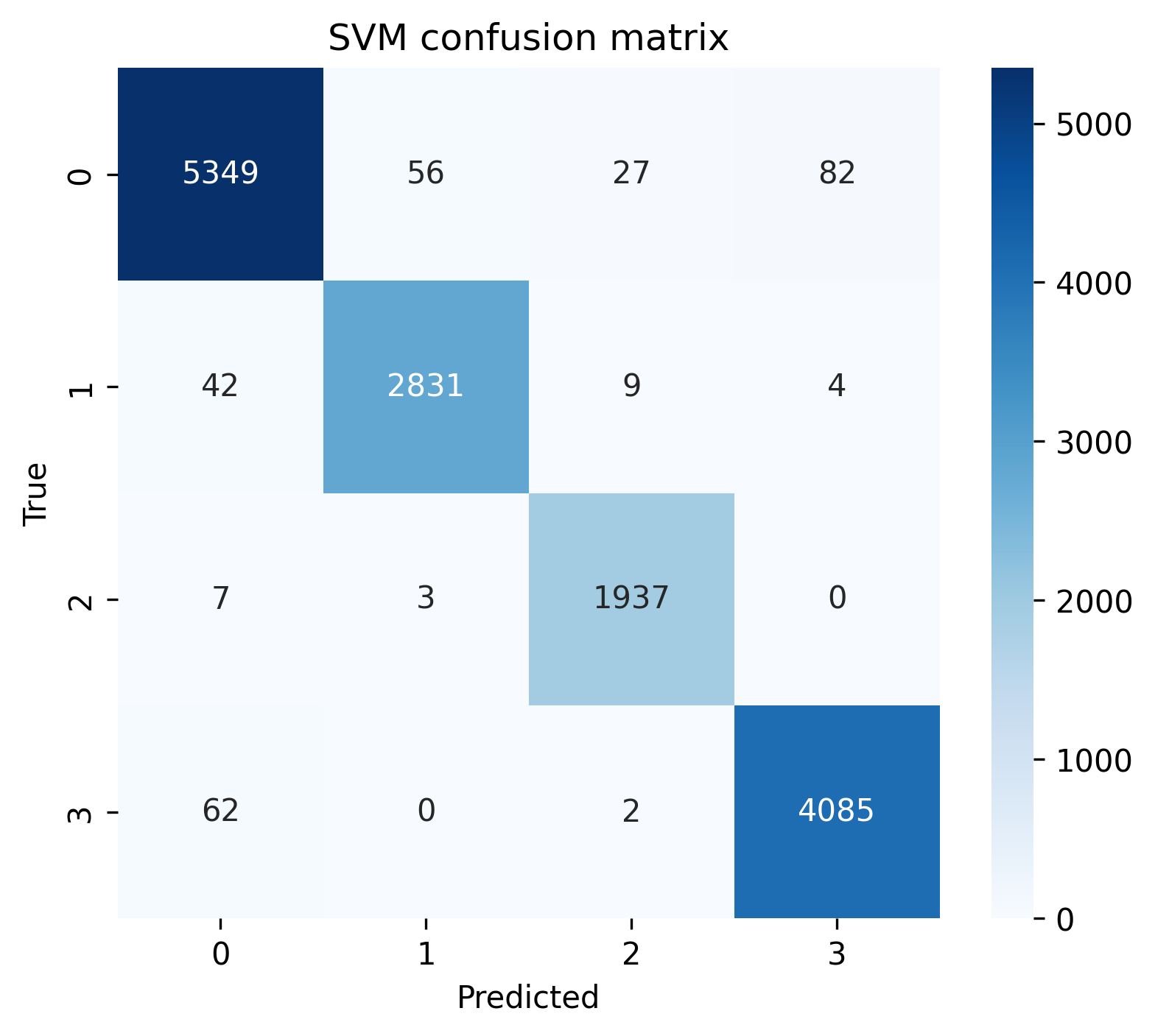
This confusion matrix for the SVM model provides detailed insight into prediction performance across the four job clusters. The diagonal elements represent correct classifications, showing the model’s impressive accuracy: 5,349 correct predictions for cluster 0, 2,831 for cluster 1, 1,937 for cluster 2, and 4,085 for cluster 3.

The off-diagonal elements reveal misclassifications. Cluster 0 has the highest number of misclassifications, with 82 samples incorrectly predicted as cluster 3, 56 as cluster 1, and 27 as cluster 2. Cluster 3 shows some confusion with cluster 0 (62 samples). Clusters 1 and 2 demonstrate minimal misclassifications, with cluster 2 having almost perfect separation (only 10 total misclassifications).

Overall, we can find that the model particularly excels at identifying clusters 1 and 2, while showing slight confusion between clusters 0 and 3. This suggests that while all clusters are well-defined by their TF-IDF features, there may be some overlapping characteristics between job descriptions in clusters 0 and 3 that occasionally cause misclassification.

Keyword heat visualization (according to the term frequency)

import numpy as np
import pandas as pd
import plotly.express as px

# Extract the vocabulary and matrix of the TF-IDF
terms = tfidf_vectorizer.get_feature_names_out()
tfidf_matrix = X_tfidf.toarray()

# Sort by word frequency
term_frequencies = tfidf_matrix.sum(axis=0)
freq_df = pd.DataFrame({'term': terms, 'frequency': term_frequencies})
freq_df = freq_df.sort_values(by='frequency', ascending=False).head(30)

# Visualize word frequency
fig = px.bar(freq_df, x='term', y='frequency', title="📈 Top 30 high-frequency words (by word frequency)", text_auto='.2s')
fig.update_layout(xaxis_tickangle=-45)
fig.write_html("./images/Top30_high_frequency.html")
fig.show()

This bar chart displays the top 30 most frequently occurring words in job descriptions, ranked by frequency. “Data” is overwhelmingly the most common term, appearing approximately 10000 times, which is nearly 4,000 occurrences more than the second-ranked word “experience” (6100). Other prominent terms include “business” (5400), “sap” (4800), and “job” (4400). The chart shows a steep decline in frequency after the top six words, with words ranking 7th through 30th ranging from about 3400 to 2100 occurrences. The prevalence of technical terms like “data”, “skills”, and “analysis” alongside business and management terminology suggests these job listings are predominantly for data-related roles requiring both technical capabilities and business acumen.

References

Khan, M., G. M. N. Islam, P. K. Ng, A. A. Zainuddin, C. P. Lean, J. Al-Fattah, A. B. Basri, and S. I. Kamarudin. (2024): “Exploring Salary Trends in Data Science, Artificial Intelligence, and Machine Learning: A Comprehensive Analysis,” AIP conference proceedings,. 1AIP Publishing.

Quan, T. Z., and M. Raheem. (2023): “Human resource analytics on data science employment based on specialized skill sets with salary prediction,” International Journal of Data Science, 4, 40–59.